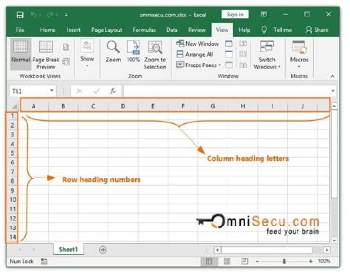
Where is heading 2 Excel?
Besides, how do you insert a heading 2?
Add a heading
- Select the text you want to use as a heading.
- On the Home tab, move the pointer over different headings in the Styles gallery. Notice as you pause over each style, your text will change so you can see how it will look in your document. Click the heading style you want to use.
Also, where are the heading styles in Excel? Select the cells that you want to format. For more information, see Select cells, ranges, rows, or columns on a worksheet. On the Home tab, in the Styles group, click the More dropdown arrow in the style gallery, and select the cell style that you want to apply.
Similarly, it is asked, what is Accent 2 Excel?
on the ribbon/toolbar are actually shortcuts to an in-built cell style. Right-click on a style, say 40% Accent 2 in pink and choose 'Modify Style' to see what it does. As you can see, this style only applies Font and Fill attributes to the cell.
Where is the Heading 1 in Excel?
On the Insert tab, in the Text group, click Header & Footer. Excel displays the worksheet in Page Layout view. To add or edit a header or footer, click the left, center, or right header or footer text box at the top or the bottom of the worksheet page (under Header, or above Footer). Type the new header or footer text.
Related Question Answers
What is the difference between Heading 1 and Heading 2 in Word?
Usually, the topic heading at the top of your page will be Heading 1. The headings of sections within the document will have Heading 2 styles. Next, give each section of the document a meaningful heading. Assign each of these a Heading 2 style.How do I apply Heading 2 style in Excel?
Apply a cell style- Select the cells that you want to format. For more information, see Select cells, ranges, rows, or columns on a worksheet.
- On the Home tab, in the Styles group, click Cell Styles.
- Click the cell style that you want to apply.
How do you get heading 2 to follow heading 1?
Click 2 in the left bar under Click level to modify, Select Heading 2 from the Link level to style drop down list, Select Level 1 from the Level to show in gallery drop down list.Why can't I find Heading 2 in Word?
Click Options and setSelect styles to show as Recommended. Click OK. Now click the right-most of the three buttons (Manage Styles). On the Recommend tab, select Heading 2 from the list and then click the Show button below.How do you continue numbering in headings?
Continuing Your Numbering- Enter the first portion of your numbered list and format it.
- Enter the heading or paragraph that interrupts the list.
- Enter the rest of your numbered list and format it.
- Right-click on the first paragraph after the list interruption.
- Choose Bullets and Numbering from the Context menu.
What are the Excel formulas?
Seven Basic Excel Formulas For Your Workflow- =SUM(number1, [number2], …)
- =SUM(A2:A8) – A simple selection that sums the values of a column.
- =SUM(A2:A8)/20 – Shows you can also turn your function into a formula.
- =AVERAGE(number1, [number2], …)
- =AVERAGE(B2:B11) – Shows a simple average, also similar to (SUM(B2:B11)/10)
Where is AutoFit in Excel?
Change the column width to automatically fit the contents (AutoFit)- Select the column or columns that you want to change.
- On the Home tab, in the Cells group, click Format.
- Under Cell Size, click AutoFit Column Width.
How do I turn on AutoCorrect in Excel?
Click File > Options > Proofing >AutoCorrect Options.How do you do linear trends in Excel?
Calculate trends by adding a trendline to a chart- Click the chart.
- Click the data series to which you want to add a trendline or moving average.
- On the Layout tab, in the Analysis group, click Trendline, and then click the type of regression trendline or moving average that you want.
What is the total cell style in Excel?
The total cell style feature in Excel 2010 makes it easy and quick for you to create professional and presentable data without having to manually highlight and format all the cells.How do you expand cell styles in Excel?
- Click the Cell Styles button. Right-click the style you want to modify, and then click Modify.
- In the Style dialog box, modify the name of your style and select the elements to include in the style.
- Click the Format button.
- Use the controls in the Format Cells dialog box to define your style.
- Click OK.
How do you do Percentage styles in Excel?
On the Home tab, in the Number group, click the icon next to Number to display the Format Cells dialog box. In the Format Cells dialog box, in the Category list, click Percentage.How do you format headings in Excel?
On the status bar, click the Page Layout View button. Select the header or footer text you want to change. On the Home tab in the Font group, set the formatting options that you want to apply to the header / footer. When you're done, click the Normal view button on the status bar.What is absolute reference in Excel?
Unlike relative references, absolute references do not change when copied or filled. You can use an absolute reference to keep a row and/or column constant. An absolute reference is designated in a formula by the addition of a dollar sign ($) before the column and row.What is Sparkline in Excel?
A sparkline is a tiny chart in a worksheet cell that provides a visual representation of data. Use sparklines to show trends in a series of values, such as seasonal increases or decreases, economic cycles, or to highlight maximum and minimum values.How do I use Quick Style in Excel?
You can Quick Style selecting the shape and then selecting a new Quick Style (on the Home tab, in the Shape Styles group, click More, and then select another Quick Style from the gallery).What is accent in Excel?
There may be times when you need to identify the formulas in an Excel worksheet. Excel provides a simple way of displaying formulas in the cells in addition to the formula bar. To display formulas in cells containing them, press the Ctrl + ` (the grave accent key is to the left of the 1 key at the top of the keyboard).How do I change the style in Excel?
Excel includes several built-in styles that you can apply or change.Change an existing cell style
- On the Home tab, click Cell Styles.
- Hold down CONTROL , click the style that you want to change, and then click Modify.
- Click Format.
- Click each tab, select the formatting that you want, and then click OK.
How do I rotate cells in Excel?
Align or rotate text in a cell- Select a cell, row, column, or a range.
- Select Home > Orientation. , and then select an option. You can rotate your text up, down, clockwise, or counterclockwise, or align text vertically:
How do I select the first 5 letters in Excel?
=LEFT (A2, 5) and press Enter on the keyboard. The function will return the first 5 characters from the cell.How do I change one heading in Excel?
In our example, we'll apply a new cell style to our existing title and header cells. Select the cell(s) you want to modify. Click the Cell Styles command on the Home tab, then choose the desired style from the drop-down menu. In our example, we'll choose Accent 1.How do I hide the header in Excel?
Show or hide the Header Row- Click anywhere in the table.
- Go to the Table tab on the Ribbon.
- In the Table Style Options group, select the Header Row check box to hide or display the table headers.
Where is the short date format in Excel?
Short Date Format in Excel- Excel provides different ways of displaying dates, be it short date, long date or a customized date.
- Click Home tab, then click the drop-down menu in Number Format Tools.
- Select Short Date from the drop-down list.
- The date is instantly displayed in short date format m/d/yyyy.
How do you make a header without changing the font?
If you want the Heading style to apply a particular font, then you have to modify the font setting in the Heading style. If you don't want to change the font in the Heading style, then your only alternatives would be to resort to direct formatting or a character style on top of the heading text.How do I use concatenate in Excel?
Here are the detailed steps:- Select a cell where you want to enter the formula.
- Type =CONCATENATE( in that cell or in the formula bar.
- Press and hold Ctrl and click on each cell you want to concatenate.
- Release the Ctrl button, type the closing parenthesis in the formula bar and press Enter.